Introduction

There are several ways in which HF propagation can be studied using a fixed frequency SSB receiver (as opposed to a swept or multi-frequency arrangement). There are broadly two types of measurement:

• Time Domain (pulse and chirped radar, digital sequence types)
• Frequency Domain (Doppler carrier measurement)

The ZL2AFP STANAG 4285 Receiver is interested only in the header which accompanies each frame of data. The transmissions are PSK, at 2400 bps, with a sub-carrier frequency of 1800 Hz. The baseband signal spans 600 to 3000 Hz, but can be adequately received with a 2.4 kHz bandwidth receiver. Each block contains 256 bits, so the frame rate is 256/2400 = 9.375 frames/sec.

We are interested only in the 80-bit header which accompanies each frame. This contains about two and a half repeats of a 31-bit Pseudo-Random Binary Sequence (P-N sequence), which in the NATO application is used to align the data before demodulation, as a means of avoiding data errors induced by propagation effects. The P-N sequence has the interesting property that when cross-correlated (compared bit-wise with a copy of the known sequence), the output is zero at all times (relative to the frame timing) except the correct one, and is a maximum when the timing matches, allowing the receiver to locate the data to within 1/256 of the correct point (about 0.4 milliseconds).

A typical Correlation from a reasonably strong signal. Note the three peaks,
the strongest in the middle, and less than average noise between the peaks.

The ZL2AFP STANAG 4285 Receiver uses the header information to study the propagation effects. The program locates and makes measurements on this P-N sequence using a very sensitive cross-correlation technique. The program is able to measure both the timing and the frequency of the transmission, and plots both the timing (propagation delay) and frequency (Doppler shift and drift). Furthermore, it includes a clever display developed by Peter Martinez G3PLX, called a Scattergram, which displays timing and frequency effects in the one image. You can make movies of the 3D Scattergram plots! The software will operate with MILITARY transmissions (1800 Hz subcarrier) and AMATEUR transmissions (1500 Hz subcarrier).

The Program

The program consists of several panes, some controls and a menu. These are shown in the picture below, and will be explained:

Correlation
The tall thin pane on the left shows the performance of the Cross-Correlator, and is called the Correlation pane. You can see that the blue line has several peaks (it is more obvious while watching the live program). These peaks are surrounded by a quiet patch (if the signal is strong), while the rest of the Correlation will be noisy. There will be three peaks, and the user chooses a point just below the centre one (as shown by the red line). There is one strong peak and two weaker peaks, because the P-N sequence is repeated about two and a half times.

Correlogram
The pane at the top is a Correlogram, which depicts changes in timing over the duration of reception. The vertical axis is time, as indicated, with an approximate distance equivalent in parentheses. You can see two faint groups of lines, spaced about 13 ms apart. This is because the span of the chart is greater than the 13 ms spacing between the P-N sequence correlation peaks. The lines of interest are the ones near 0 ms. If the signal is within ground wave range, there will be a strong and very clean line which ideally should be set to zero on the Correlogram. The Correlogram moves along in time, with time marked underneath. The speed and averaging of the chart can be adjusted.

Dopplergram
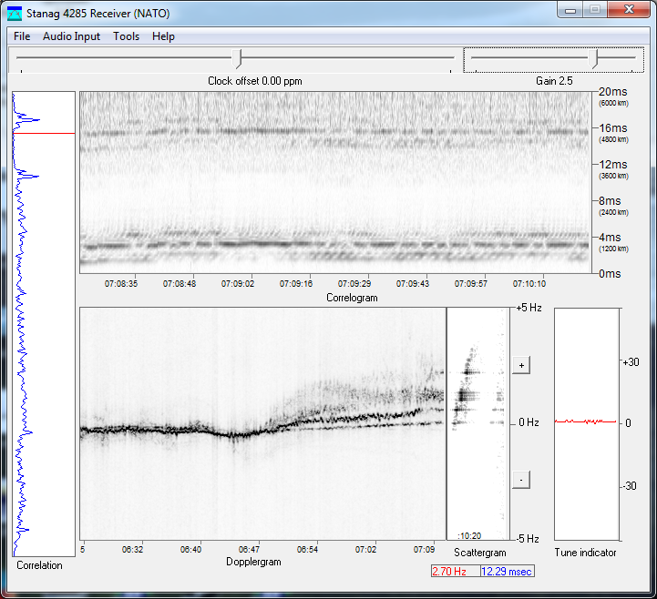
The pane below the Correlogram, with a dark background, is the Dopplergram, which shows frequency variations in the received signal. In this example, recorded at about sunrise, there are several frequency products visible. At the right of this pane, you see (as the lowest line) the E-layer response, and above that the F1 and F2 responses, followed by double-hop F1 and F2 responses, plus scatter. The double-hop returns are generally only seen at sunrise, and represent rays of the signal that have been returned from the F layer, bounced off the earth, then again returned by the F layer. These are characterised by double the Doppler shift of the main F layer returns, and are weaker due to loss, particularly on reflection from the earth. The height of the Dopplergram is ±5 Hz, and the Dopplergram moves along in time, with time marked underneath.

Scattergram
To the right of the Dopplergram is the Scattergram, which is a unique combination of frequency and timing, and slowly changes with time. As you can see, the vertical axis of the Scattergram exactly matches that of the Dopplergram, and shows (averaged) the exact same frequency effects seen on the latter. The horizontal axis of the Scattergram is propagation time. Zero at the left and about 16 ms on the right, so you can easily read off the additional time-of-flight and frequency shift of the various products with remarkable precision (0.25 ms and 0.04 Hz resolution).

In the example picture above, there is a whole line of products stretching up in frequency as far as +3 Hz, and +10 ms. For the first time, we can recognise and measure these individual products. Note how the individual dots are roughly in a straight line and some are very sharp. The increase in frequency is caused by Doppler shift, as at sunrise the apparent height of each layer moves closer to earth with increasing refractive index (ion density). Below the Scattergram is a small box, in which the frequency offset and delay are indicated when the mouse is hovered over a point on the Scattergram.

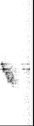
Here are two examples of Scattergrams of the same station on 4.5 MHz, morning and evening, at a range of about 1000 km. The ionosphere is much more disturbed in the evening after being stimulated all day, which causes increased scatter (looks like noise). It settles down overnight. The first picture was captured at sunrise, the second at sunset.

       
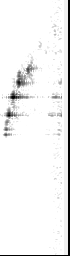
Sunrise                     Sunset

In the first picture you can clearly see the E-layer return (sharp dot with least delay) other minor dots, (possibly reflections off aircraft), then two strong dots, which are the F1 and F2 returns, followed by another two, which are double-hop F1 and F2. These have double the shift because they have been returned twice from the ionosphere and of course have increased delay. The dots are in a line of increasing frequency, as the active height of the layers is reducing with increasing ion density and therefore increasing refractive index.

In the evening the E and F returns are strong, and there are scattered (and therefore indistinct) returns from the F layer, probably from points not on the direct path. The dots and scatter are in a line of decreasing frequency, as the active height of the layers is increasing as the charged ions slowly disippate.

It is important to use a very stable synthesised receiver and a good antenna to achieve results like this. The Scattergrams are only 10 Hz high.